[ML][EN]Sparse Encoder

Neural Network in a nutshell

This post was written by referring Andrew Ng’s lec note in Stanford University

0. Found at

• Paper : Andrew Ng CS294A Lecture notes https://web.stanford.edu/class/cs294a/sparseAutoencoder_2011new.pdf

1. AutoEncoder and Sparsity

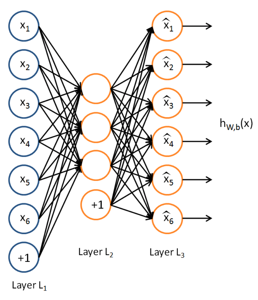
Suppose we have only unlabeled training examples set. An AutoEncoder neural network is an unsupervised learning algorithm that applies backpropagation, setting the target values to be equal to the inputs. I.e., it uses $y^{(i)}=x^{(i)}$

1.1. Diagram

Main Concept

As autoencoder set target values to be equal to the inputs, it tries to learn a function $h_{W, b}(x) = \hat{x} \approx x$

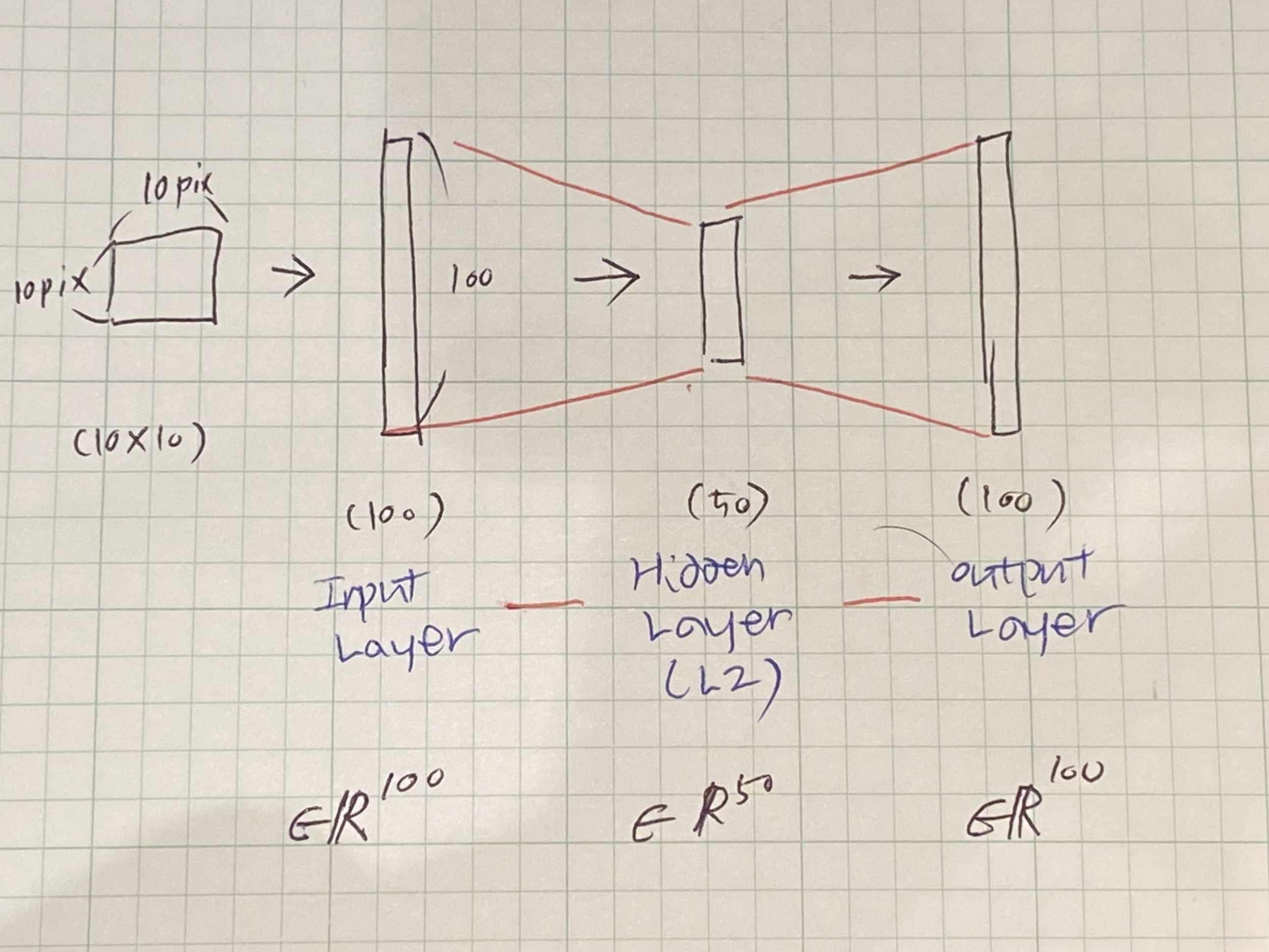
Let’s assume, we are training 100 pixels(10 by 10) images and put hidden layer in $L_2$ which has 50 units(neurons). That is, the constraints on the network is implemented. Through this, we can discover interesting structure about the data.

Here, inputs $x$ are 100 pixels image so $n = 100$. Then, for autoencoding, 50 units were implemented which is, $s_2 = 50$, to layer $L_2$. As output ought to be 100 pixels, $y \in \mathbb{R}^{100}$, with no doubt.

• Key idea
  

Parameters(or each $x_i$) are set IID Gaussian independent. Compress from 100 to 50 would be very very difficult. But if there is structure in the data, same to say ‘some of the input features are correlated’, then this algorithm can discover some of those correlatoins. That is the key idea of autoencoding

• Sparsity Implemented
  

There is the case the number of units in the hidden layer is larger than that in the input layer, here $s_2 = 200$. Still, we can discover interesting structure. In particular, if we impose SPARSITY constraints on the $s_2$, the autoencoder can discover the interesting structure in the data, even the number of hidden units is large.

1.2. Kullback–Leibler divergence

• Neuron is “active/firing” or “inactive”
  

for SIGMOID activation function, Neuron is considered “active” or “firing” when its outvalue is close to 1.
Neuron is considered “inactive” when its outvalue is close to 0. (If you are using a tanh activation function, then we think of a neuron as being inactive when it outputs values close to -1)

Here, we would like to constrain the neurons to be inactive most of the time.

• KL divergence
  In KL divergence, the penalty term can be written as

$\sum_{j=1}^{s_{2}} KL \left( \rho || \hat{\rho}_{j} \right)$ where

$\rho$ : Bernoulli random variable with mean $\rho$
$\hat{\rho}$ : Bernoulli random variable with mean $\hat{\rho}$

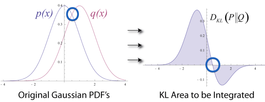
KL diversion, which is abbreviation of Kullback–Leibler divergence, is a measure of how one probability distribution is different from a second, reference probability distribution. We got two Bernoulli random variable($\rho, \hat{\rho}$) and then eager to compare the distribution by gauging relative entropy of the two.

To simplify KL divergence, intuitively, (SEE LEFT)two distribution $p(x), q(x)$ shapes similar(guess the same) but have small difference in the mean. Gaussian Distribution $p(x)$ has mean of ‘0’. Probability on the right hand side of $x=0$ decreases while $q(x)$ is not. And they have same prob at $x\approx 0.4$ (SEE RIGHT) If two mean is the same, divergence is zero and can be seen in blue circle. To say by formula, \(\mathrm{KL}\left(\rho \| \hat{\rho}_{j}\right)=0\) if $\hat{\rho}_{j}=\rho$

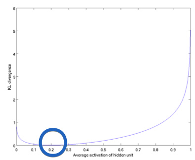
We have set $\rho = 0.2$ and plotted \(\mathrm{KL}\left(\rho \| \hat{\rho}_{j}\right)\) for a range of values of . and we see that KL-divergence reaches its minimun(blue circle) at $\hat{\rho}_{j}=\rho$ and blows up as it approaches to 1.
Thus, minimizing this penalty term has the effect of causing $\hat{\rho}$ to be close to $\rho$
Then, overall cost function is now

$J_{\text {sparse }}(W, b)=J(W, b)+\beta \sum_{j=1}^{s_{2}} \mathrm{KL}\left(\rho | \hat{\rho}_{j}\right)$ where $\beta$ controls the weight of the sparsity penalty term.
The term $\hat{\rho}$ implicitly depends on $W, b$ also, beacuse it is the average activation of hidden unit $j$, and the activation of a hidden unit depends on the parameters $W,b$.
To apply KL-divergence to error term function, we retrieve that we backpropagated as below.

$\delta_{i}^{(2)}=\left(\sum_{j=1}^{s_{2}} W_{j i}^{(2)} \delta_{j}^{(3)}\right) f^{\prime}\left(z_{i}^{(2)}\right)$
now instead we compute,

$\delta_{i}^{(2)}=\left(\left(\sum_{j=1}^{s_{2}} W_{j i}^{(2)} \delta_{j}^{(3)}\right)+\beta\left(-\frac{\rho}{\rho_{i}}+\frac{1-\rho}{1-\rho_{i}}\right)\right) f^{\prime}\left(z_{i}^{(2)}\right)$

if we implement the autoencoder using backpropagation modified this way, you will be performing gradient descent exactly on the objective $J_{\text {sparse }}(W, b)$.

2. Visualization

Consider the case of training autoencoer on 10 X 10 images, so that $n = 100$. Each hidden unit $i$ computes a function of input:

Reference

• Kullback–Leibler divergence(wikipedia): https://en.wikipedia.org/wiki/Kullback%E2%80%93Leibler_divergence#Definition

Not The End

• 2020 21