[ML][EN]Neural Network

Neural Network in a nutshell

This post was written by referring Andrew Ng’s lec note in Stanford University

0. Found at

• Paper : Andrew Ng CS294A Lecture notes https://web.stanford.edu/class/cs294a/sparseAutoencoder_2011new.pdf

1. Neural Networks

Considering supervised learning problem, where we have access to labeled training examples, NN give a way defining a complex, non-linear form of hypotheses $h_{W, b}(x)$, with parameters W,b that we can fit to our data.

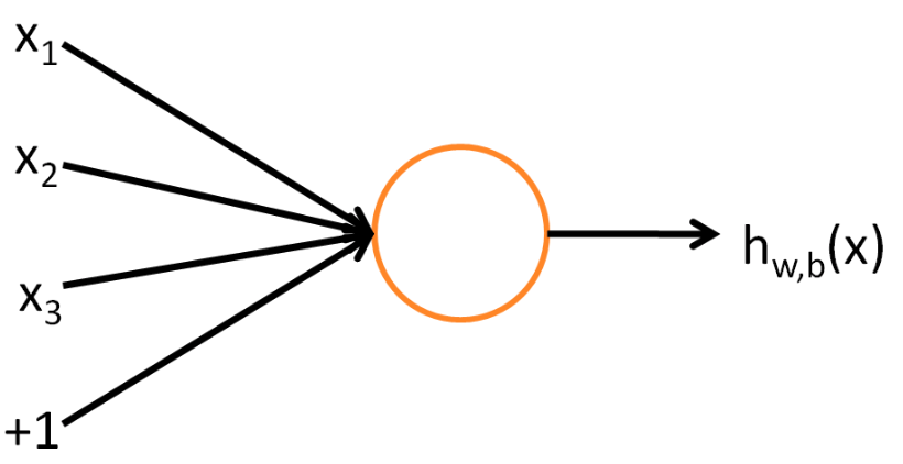
To describe neural networks, we will begin by describing the simplest possible neural network, one which comprises a single “neuron.”(orange circle)

• input : $x_1$, $x_2$, $x_3$, $x_4$, $+1$(=bias unit, intercept term)
• medium : neuron
• output : $h_{W, b}(x)=f\left(W^{T} x\right)=f\left(\sum_{i=1}^{3} W_{i} x_{i}+b\right)$

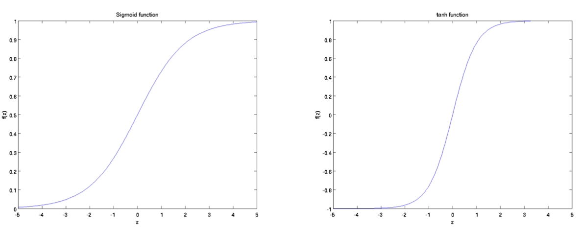
Here, $f(\cdot)$ is called activation and sigmoid function will be it:

$f: \mathbb{R} \mapsto \mathbb{R}$ and $f(z)=\frac{1}{1+\exp (-z)}$

It is worth noting another activation function which is called hyperbolic tangent, or tanh function:

$f: \mathbb{R} \mapsto \mathbb{R}$ and $f(z)=\tanh (z)=\frac{e^{z}-e^{-z}}{e^{z}+e^{-z}}$

Plots of two activation function is as below. The tanh(z) function is a rescaled version of the sigmoid, and its output range is [−1, 1] instead of [0, 1].

To notify, it’s also worth noting that If $f(z)=1 /(1+\exp (-z))$ is the sigmoid function, then its derivative is given by $f^{\prime}(z)=f(z)(1-f(z))$. (If $f$ is the tanh function, then its derivative is given by $f^{\prime}(z)=1-(f(z))^{2}$) You can derive this yourself using the definition of the sigmoid (or tanh) function.

1.1. Neural Networks Formulation

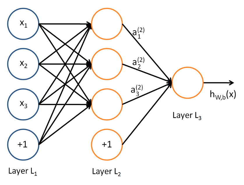
• Layer $L_1$ → “Input Layer” $x_1$, $x_2$, $x_3$, $x_4$, $+1$(=bias unit, intercept term)
• Layer $L_2$ → “Hidden Layer” - values not observed in training set $h_1$, $h_2$, $h_3$, $h_4$, $+1$(=bias unit, intercept term)

• Formulation → NN(Neural Networks) has 3 input units, 3 hidden units and 1 output unit

Denote

• $n_l$ → # of layer in NN
• $l$ → label layer
• $L_1$ → input layer , $L_{n_{l}}$ → output layer
• $W_{i j}^{(l)}$ → parameter(weight) associated with the connection between [unit $j$ in layer $l$] and [unit $i$ in layer $l+1$]
• $b_{i}^{(l)}$ → bias associated with unit $i$ in layer $l+1$

• $s_l$ → # of nodes in the layer $l$

• $(W,b) = \left(W^{(1)}, b^{(1)}, W^{(2)}, b^{(2)}\right)$

• $a_{i}^{(l)}$ → the activation of unit $i$ in layer $l$ (for $l = 1$, $a_{i}^{(1)}=x_{i}$)

• $f(\cdot)$ → the activation function

Then, the computation of NN is given by:

$\begin{aligned} a_{1}^{(2)} &=f\left(W_{11}^{(1)} x_{1}+W_{12}^{(1)} x_{2}+W_{13}^{(1)} x_{3}+b_{1}^{(1)}\right) —(2) \cr\cr a_{2}^{(2)} &=f\left(W_{21}^{(1)} x_{1}+W_{22}^{(1)} x_{2}+W_{23}^{(1)} x_{3}+b_{2}^{(1)}\right) —(3)\cr\cr a_{3}^{(2)} &=f\left(W_{31}^{(1)} x_{1}+W_{32}^{(1)} x_{2}+W_{33}^{(1)} x_{3}+b_{3}^{(1)}\right) —(4)\cr\cr h_{W, b}(x) &=a_{1}^{(3)}=f\left(W_{11}^{(2)} a_{1}^{(2)}+W_{12}^{(2)} a_{2}^{(2)}+W_{13}^{(2)} a_{3}^{(2)}+b_{1}^{(2)}\right) —(5)\end{aligned}$

Here, let $z_{i}^{(l)}$ be the total weighted sum of inuts to unit $i$ in layer $l$(eg. $z_{i}^{(2)}=\sum_{j=1}^{n} W_{i j}^{(1)} x_{j}+b_{i}^{(1)}$), including bias term written as $b$, so that $a_{i}^{(l)}=f\left (z_{i}^{(l)}\right)$

If we extend the activation function $f(\cdot)$ to apply vectors in element wise function (eg. $f\left(\left[z_{1}, z_{2}, z_{3}\right]\right)=\left[f\left(z_{1}\right), f\left(z_{2}\right), f\left(z_{3}\right)\right]$ ), then we can write equation $(5)$ more easily as:

$\begin{aligned} z^{(2)} &=W^{(1)} x+b^{(1)} \cr\cr a^{(2)} &=f\left(z^{(2)}\right)\cr\cr z^{(3)} &=W^{(2)} a^{(2)}+b^{(2)} \cr\cr h_{W, b}(x) &=a^{(3)}=f\left(z^{(3)}\right) \end{aligned}$

And recalling that values of input layer can be written as $a^{(1)}=x$, we can compute layer $l+1$’s activations $a^{(l+1)}$ as:

$\begin{aligned} z^{(l+1)} &=W^{(l)} a^{(l)}+b^{(l)} —(6)\cr\cr a^{(l+1)} &=f\left(z^{(l+1)}\right) —(7) \end{aligned}$

By organizing parameters in matrices using matrix-vector operations, we can take the advantage of easiness / fastdness of linear algebra routines to quickly perform calculations in network.

Feed Forward network

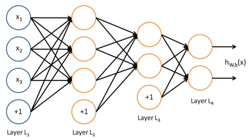
In this setting, to compute the output of the network, we can successively compute all the activations in layer $L_2$, then layer $L_3$, and so on, up to layer $L_{nl}$ , using Equations (6) and (7). This is one example of a feed forward neural network, since the connectivity graph does not have any directed loops or cycles. Neural networks can also have multiple output units. For example, here is a network with two hidden layers layers $L_2$ and $L_3$ and two output units in layer $L_4$

1.2. Backpropagation algorithm

Suppose we have $m$ training example with {($x^{1}$ ~ $x^{m}$), ($y^{1}$ ~ $y^{m}$)}. Here we can define loss(cost) function with one half squared-error function

$J(W, b ; x, y)=\frac{1}{2}\left|h_{W, b}(x)-y\right|^{2}$

Then, the overall cost function is

$\begin{aligned} J(W, b) &=\left[\frac{1}{m} \sum_{i=1}^{m} J\left(W, b ; x^{(i)}, y^{(i)}\right)\right]+\frac{\lambda}{2} \sum_{l=1}^{n_{l}-1} \sum_{i=1}^{s_{l}} \sum_{j=1}^{s_{l+1}}\left(W_{j i}^{(l)}\right)^{2} \cr\cr &=\left[\frac{1}{m} \sum_{i=1}^{m}\left(\frac{1}{2}\left|h_{W, b}\left(x^{(i)}\right)-y^{(i)}\right|^{2}\right)\right]+\frac{\lambda}{2} \sum_{l=1}^{n_{l}-1} \sum_{i=1}^{s_{l}} \sum_{j=1}^{s_{l+1}}\left(W_{j i}^{(l)}\right)^{2} \cr\cr —(8)\end{aligned} $

Here,

• $J(W, b)$ : An average of sum-of-squares error term
• $\lambda$ : Lambda is weight decay parameter which prevents overfitting by decreading the magnitude of the weights.

Our Goal is to minimize $J(W, b)$ as a function of $W$ and $b$.

To train our neural network, we will initialize each parameter $W_{i j}^{(l)}$ and each $b_{i}^{(l)}$ to a small random value near zero and then apply an optimazation algorithm such as batch gradient descent. Note that it is important to initialize the parameters randomly, rather than to all 0’s. Here the random initialization serves the purpose of symmetry breaking. Iteration of gradient descent updates the parameters as written as:

$\begin{aligned} W_{i j}^{(l)} &:=W_{i j}^{(l)}-\alpha \frac{\partial}{\partial W_{i j}^{(l)}} J(W, b) \cr\cr b_{i}^{(l)} &:=b_{i}^{(l)}-\alpha \frac{\partial}{\partial b_{i}^{(l)}} J(W, b) \end{aligned}$ where $\alpha$ is learning rate.

Backpropagation Algorithm

Backpropagation Algorithm is an efficient way to compute partial derivatives above. Using Equation $(8)$, we can see that overall cost function $J(W, b)$ can be calculated as:

$\begin{aligned} \frac{\partial}{\partial W_{i j}^{(l)}} J(W, b) &=\left[\frac{1}{m} \sum_{i=1}^{m} \frac{\partial}{\partial W_{i j}^{(l)}} J\left(W, b ; x^{(i)}, y^{(i)}\right)\right]+\lambda W_{i j}^{(l)} \cr\cr \frac{\partial}{\partial b_{i}^{(l)}} J(W, b) &=\frac{1}{m} \sum_{i=1}^{m} \frac{\partial}{\partial b_{i}^{(l)}} J\left(W, b ; x^{(i)}, y^{(i)}\right) \end{aligned}$

(note that weight decay $\lambda$ is applied to $W$(weight) but not to $b$(bias))

Given training example $(x, y)$, we first run “forward pass” to compute all activations in neural network, including the output value of hypothesis $h_{W, b}(x)$.
Then for each node $i$ in layer $l$, we calculate an “error term” $\delta_{i}^{(l)}$ measuring how much that node was “responsible” for any errors in our output

Step

1. Perform a feedforward pass, computing the activations for layers $L_2$, $L_3$, …, and so on up to the output layer $L_{nl}$

2. For each output unit $i$ in layer $n_l$ (the output layer), set $\delta_{i}^{\left(n_{l}\right)}=\frac{\partial}{\partial z_{i}^{\left(n_{l}\right)}} \frac{1}{2}\left|y-h_{W, b}(x)\right|^{2}=-\left(y_{i}-a_{i}^{\left(n_{l}\right)}\right) \cdot f^{\prime}\left(z_{i}^{\left(n_{l}\right)}\right)$

3. For $l=n_{l}-1, n_{l}-2, n_{l}-3, \ldots, 2$, For each node $i$ in layer $l$, set
   $\delta_{i}^{(l)}=\left(\sum_{j=1}^{s_{l+1}} W_{j i}^{(l)} \delta_{j}^{(l+1)}\right) f^{\prime}\left(z_{i}^{(l)}\right)$

4. Compute the desired partial derivatives, which are given as:
   $\begin{aligned} \frac{\partial}{\partial W_{i j}^{(l)}} J(W, b ; x, y) &=a_{j}^{(l)} \delta_{i}^{(l+1)} \cr\cr \frac{\partial}{\partial b_{i}^{(l)}} J(W, b ; x, y) &=\delta_{i}^{(l+1)} \end{aligned}$

From now on, we use $\bullet$ to denote the element-wise product operator. if $a=b \bullet c$, then it’s $a_{i}=b_{i} c_{i}$.
Extending this to the function definition $f(\cdot)$ to apply element-wise to vectors, we do the same definition for $f^{\prime}(\cdot)$ Then,
$f^{\prime}\left(\left[z_{1}, z_{2}, z_{3}\right]\right)=\left[\frac{\partial}{\partial z_{1}} f\left(z_{1}\right), \frac{\partial}{\partial z_{2}} f\left(z_{2}\right), \frac{\partial}{\partial z_{3}} f\left(z_{3}\right)\right]$

The backpropagation algorithm can then be written:

1. Perform a feedforward pass, computing the activations for layers $L_2$, $L_3$, up to the output layer $L_{nl}$, using Equations $(6-7)$.

2. For the output layer (layer $nl$), set

$\delta^{\left(n_{l}\right)}=-\left(y-a^{\left(n_{l}\right)}\right) \bullet f^{\prime}\left(z^{(n)}\right)$

1. For $l=n_{l}-1, n_{l}-2, n_{l}-3, \ldots, 2$,
   Set $\delta^{(l)}=\left(\left(W^{(l)}\right)^{T} \delta^{(l+1)}\right) \bullet f^{\prime}\left(z^{(l)}\right)$

2. Then Compute the desired partial derivatives: $\begin{aligned} \nabla_{W^{(l)}} J(W, b ; x, y) &=\delta^{(l+1)}\left(a^{(l)}\right)^{T}, \cr\cr \nabla_{b^{(l)}} J(W, b ; x, y) &=\delta^{(l+1)} \end{aligned}$

1.3. Gradient Checking and Advanced Optimization

We describe a method for numerically checking the derivatives computed by your code to make sure that your implementation is correct. Carrying out the derivative checking procedure described here will signifi- cantly increase your confidence in the correctness of your code.

In 1-D case, one iteration of gradient descent is given by:

$\theta:=\theta-\alpha \frac{d}{d \theta} J(\theta)$

where $J: \mathbb{R} \mapsto \mathbb{R},$ so that $\theta \in \mathbb{R}$ aiming for minimize $J(\theta)$ as a function of $\theta$. We say function $g(\theta)$ that purportedly computes $\frac{d}{d \theta} J(\theta)$. We should check if out implemetation of g is correct or not.

To recall the mathematical definition of the derivative as
$\frac{d}{d \theta} J(\theta)=\lim _{\epsilon \rightarrow 0} \frac{J(\theta+\epsilon)-J(\theta-\epsilon)}{2 \epsilon}$

Let us add new jargon called EPSILON. In practive, we set EPSILON to a small constant, say around $10^{-4}$(if it is smaller, it would lead to roundoff errors.)

Using EPSILON, we can numerically approximate the derivative as follows:

$\frac{J(\theta+\mathrm{EPSILON})-J(\theta-\mathrm{EPSILON})}{2 \times \mathrm{EPSILON}}$

Aforementioned, as function $g(\theta)$ that purportedly computes $\frac{d}{d \theta} J(\theta)$, we can verify its correctedness by checking that
$g(\theta) \approx \frac{J(\theta+\mathrm{EPSILON})-J(\theta-\mathrm{EPSILON})}{2 \times \mathrm{EPSILON}}$

Now, consider $\theta \in \mathbb{R}^{n}$ is vector rather than a single number(=which is, we got $n$ parameters that we want to learn) and $J: \mathbb{R}^{n} \mapsto \mathbb{R}$.

Suppose we have function $g_{i}(\theta)$ that purportedly computes $\frac{\partial}{\partial \theta_{i}} J(\theta)$, we will check if $g_{i}(\theta)$ is outputting correct derivative values.

Let

$\theta^{(i+)} = \theta+$ EPSILON $\times \vec{e}_{i}$,

$\theta^{(i-)} = \theta-$ EPSILON $\times \vec{e}_{i}$

where

$\vec{e}_{i}=\left[\begin{array}{c}0 \cr 0 \cr \vdots \cr 1 \cr \vdots \cr 0\end{array}\right]$

We can now verify $g_{i}(\theta)$ ‘s correctness by checking for each $i$, that:

$g_{i}(\theta) \approx \frac{J\left(\theta^{(i+)}\right)-J\left(\theta^{(i-)}\right)}{2 \times \text { EPSILON }}$

When implementing backpropagation to train a NN, we will have that $\begin{aligned} \nabla_{W^{(l)}} J(W, b) &=\left(\frac{1}{m} \Delta W^{(l)}\right)+\lambda W^{(l)} \ \nabla_{b^{(l)}} J(W, b) &=\frac{1}{m} \Delta b^{(l)} \end{aligned}$

Here we saw basic concept of neuron, neural networks and backpropagation algorithm. Next we will explore AutoEncoding.

The End

• 2020 21