AML Logo Design Project
Non-designer designs the design of laboratory’s symbol, interestingly.
Table of Contents
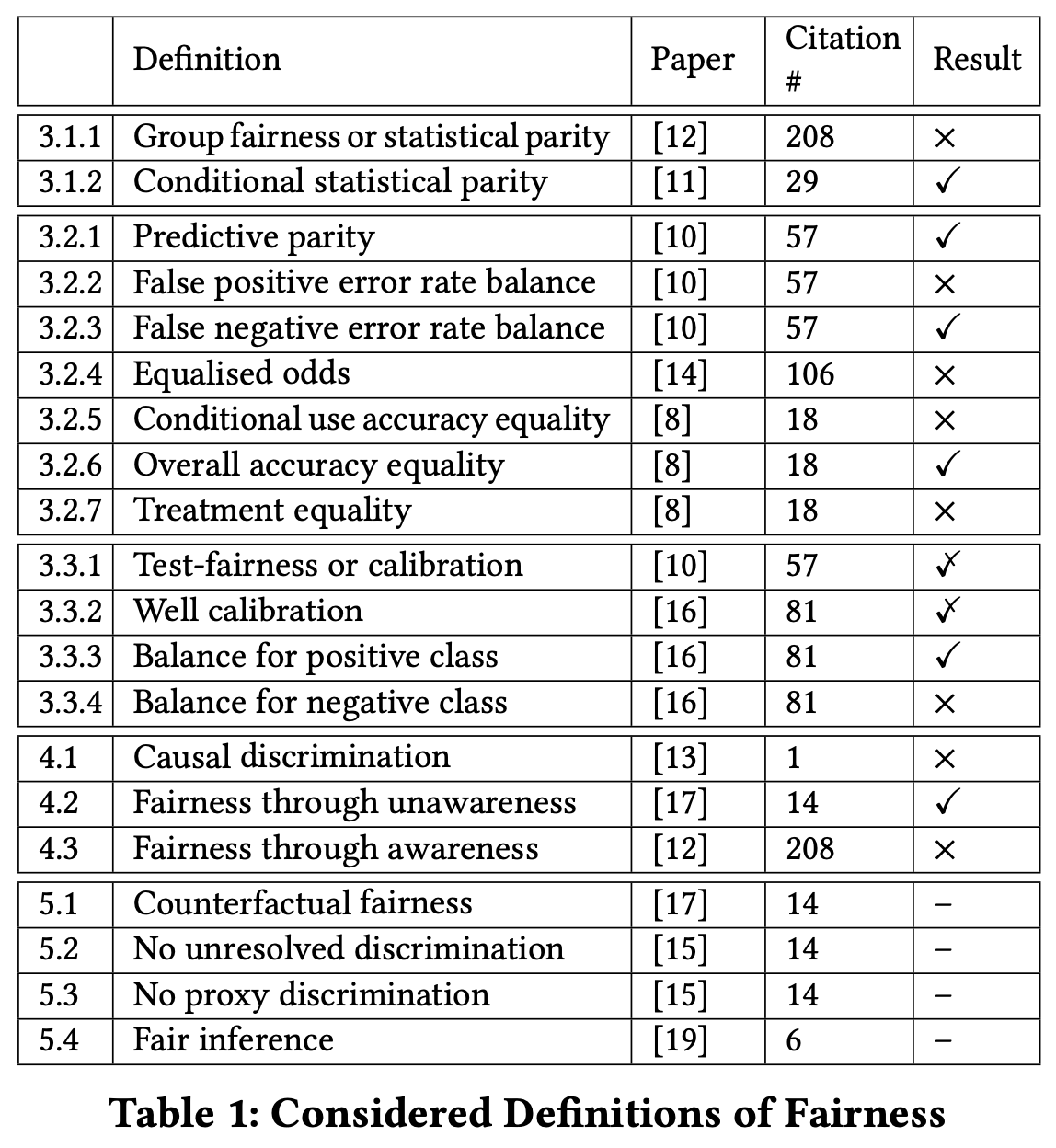
Algorithm fairness has started to attract the attention of researchers in AI, Software Engineering and Law communities, with more than twenty different notions of fairness proposed in the last few years.
Yet, there is no clear agreement on which definition to apply in each situation.
Here in the paper, it intuitively explains why the same case can be considered fair according to some definitions and unfair according to others.
AI now replaces humans at many critical decision points, such as who will get a loan [1] and who will get hired for a job [3]. One might think that these AI algorithms are objective and free from human biases, but that is not the case. For example, risk-assessment software employed in criminal justice exhibits race-related issues [4] and a travel fare aggregator steers Mac users to more expensive hotels [2]
The topic of algorithm fairness has begun to attract attention in the AI and Software Engineering research communities. In late 2016, the IEEE Standards Association published a 250-page draft docu- ment on issues such as the meaning of algorithmic transparency.
In this paper, we focus on the machine learning (ML) classification problem: identifying a category for a new observation given training data containing observations whose categories are known. We collect and clarify most prominent fairness definitions for clas- sification used in the literature, illustrating them on a common, unifying example – the German Credit Dataset This dataset is commonly used in fairness literature. It contains information about 1000 loan applicants and includes 20 attributes describing each applicant, e.g., credit history, purpose of the loan, loan amount requested, marital status, gender, age, job, and housing status. It also contains an additional attribute that describes the classification outcome – whether an applicant has a good or a bad credit score.
© Verma et al.,
Above rows are definitions of ‘fairness’. All of them are papers. We will explain and see ‘fairness’ of algorithm from German Credit Dataset.
Heading is comprised of ‘#.#.#’ and the meaning is further explained below.
3.#.# STATISTICAL MEASURES
4.# SIMILARITY-BASED MEASURES
5.# CAUSAL REASONING
For example, the probability of having a good credit score ($S$) as established by a classifier is 88%. Thus, the predicted score ($d$) is good, same as the actual credit score recorded in the database ($Y$)
© Verma et al.,
© Wikipedia
A classifier satisfies this definition if subjects in both protected and unprotected groups have equal probability of being assigned to the positive predicted class.
\[P(d=1|G=m) = P(d=1|G=f)\]where,
Applicants should have an equivalent opportunity to obtain a good credit score, regardless of their gender.
The probability to have a good predicted credit score
It is more likely for a male applicant to have good predicted score, so that we can deem classifier to fail in satisfying this definition of fairness.
Definition is satisfied if subjects in both protected and unprotected groups have equal probability of being assigned to the positive predicted class, controlling for a set of legitimate factors $L$.
As the examples of $L$, possible legitimate factors that affect an applicant creditworthiness could be the requested credit amount, applicant’s credit history, employment, and age.
\[P(d=1|L=l, G=m) = P(d=1|L=l,G=f)\]where,
The probability to have a good predicted credit score
Unlike in the previous definition, here a female applicant is slightly more likely to get a good predicted credit score.
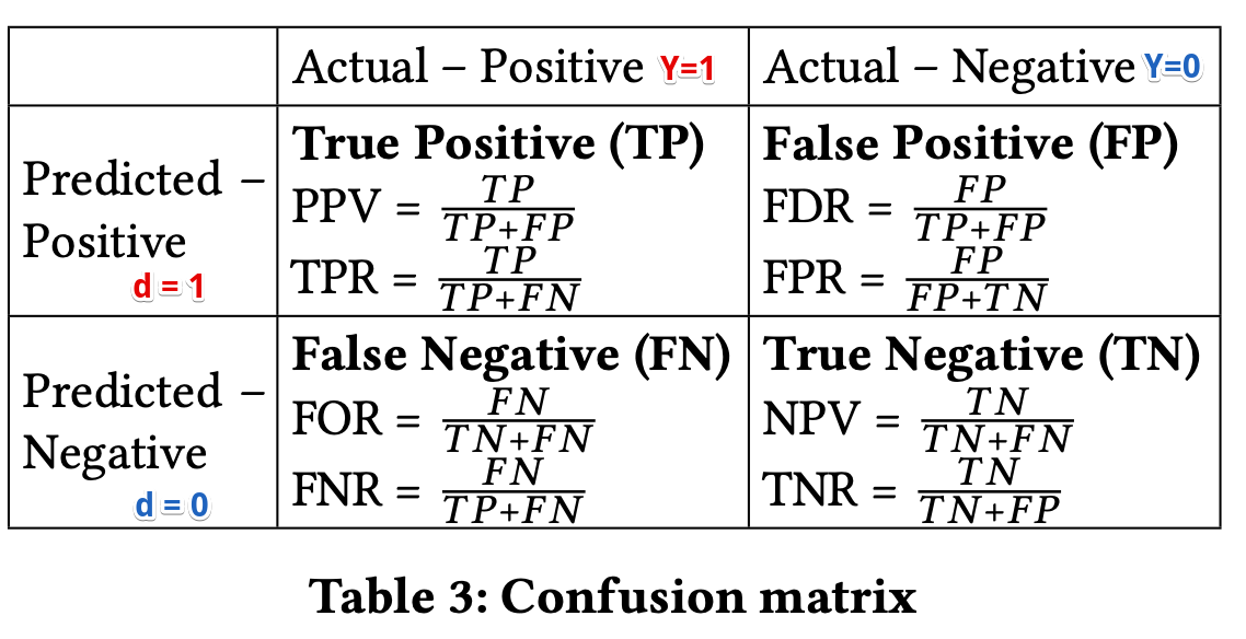
A classifier satisfies this definition if both protected and unprotected groups have equal $PPV$ – the probability of a subject with positive predictive value to truly belong to the positive class.
Main idea behind this definition is that the fraction of correct positive predictions should be the same for both genders.
\[P(Y=1|d=1,G=m) = P(Y=1|d=1,G=f)\]where,
Mathematically, a classifier with equal $PPV$s will also have equal $FDRs$ which are $P(Y = 0|d = 1,G = m) = P(Y = 0|d = 1,G = f)$.
The values are not strictly equal, but, again, we consider this difference minor, and hence deem the classifier to satisfy this definition.
A classifier satisfies this definition if both protected and unprotected groups have equal $FPR$ – the probability of a subject in the negative class to have a positive predictive value.
The main idea behind this definition is that a classifier should give similar results for applicants of both genders with actual negative credit scores.
\[P(d = 1|Y = 0,G = m) = P(d = 1|Y = 0,G = f )\]where,
Mathematically, a classifier with equal $FPR$s will also have equal $TNR$s which are $P(d = 0|Y = 0,G = m) = P(d = 0|Y = 0,G = f)$.
The classifier is more likely to assign a good credit score to males who have an actual bad credit score; females do not have such an advantage and the classifier is more likely to predict a bad credit score for females who actually have a bad credit score. Classifier is deemed to fail in satisfying this definition of fairness.
A classifier satisfies this definition if both protected and unprotected groups have equal $FNR$ – the probability of a subject in a positive class to have a negative predictive value.
This implies that the probability of an applicant with an actual good credit score to be incorrectly assigned a bad predicted credit score should be the same for both male and female applicants
\[P(d = 0|Y = 1,G = m) = P(d = 0|Y = 1,G = f )\]where,
Mathematically, a classifier with equal $FNR$s will also have equal $TPR$ which are $P(d = 1|Y = 1,G = m) = P(d = 1|Y = 1,G = f )$.
This means that the classifier will apply equivalent treatment to male and female applicants with actual good credit score. Classifier is deemed to be satisfying this definition of fairness.
Definition combines the previous two: a classifier satisfies the definition if protected and unprotected groups have
where,
$FPR$
$TPR$
This means that the classifier is more likely to assign a good credit score to males who have an actual bad credit score, compared to females. Hence the overall conjunction does not hold and we deem our classifier to fail in satisfying this definition.
Definition combines the two: a classifier satisfies the definition if protected and unprotected groups have
This definition implies equivalent accuracy for male and female applicants from both positive and negative predicted classes. In our example, the definition implies that for both male and female applicants, the probability of an applicant with a good predicted credit score to actually have a good credit score and the probability of an applicant with a bad predicted credit score to actually have a bad credit score should be the same.
\[P(Y=1|d=1,G=m)=P(Y=1|d=1,G=f))∧(P(Y= 0|d=0,G=m)=P(Y=0|d=0,G=f)\]where,
$PPV$
$NPV$
It is more likely for a male than female applicant with a bad predicted score to actually have a good credit score. We thus deem the classifier to fail in satisfying this definition of fairness.definition.
A classifier satisfies this definition if
The definition assumes that
In this example, this implies that the probability of an applicant with an actual good credit score to be correctly assigned a good predicted credit score and an applicant with an actual bad credit score to be correctly assigned a bad predicted credit score is the same for both male and female applicants.
\[P(d = Y,G = m) = P(d = Y,G = f )\]where,
While these values are not strictly equal, for practical purposes we consider this difference minor, and hence deem the classifier to satisfy this definition
This definition looks at the ratio of errors that the classifier makes rather than at its accuracy. A classifier satisfies this definition if both protected and unprotected groups have an equal ratio of false negatives and false positives.
\[\frac{FN}{FP}(m) = \frac{FN}{FP}(f)\]where,
a smaller number of male candidates are incorrectly assigned to the negative class ($FN$) and / or larger number of male candidates are incorrectly assigned to the positive class ($FP$). Classifier is deemed to fail in satisfying this definition of fairness.
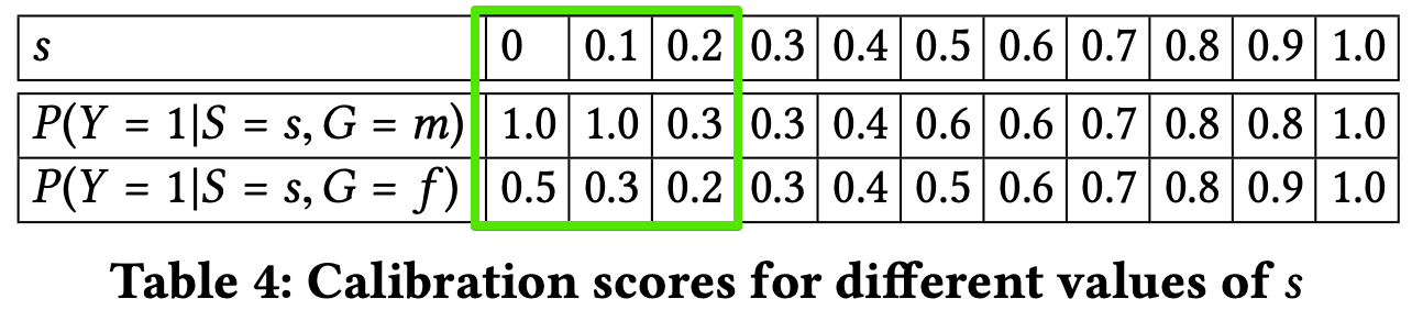
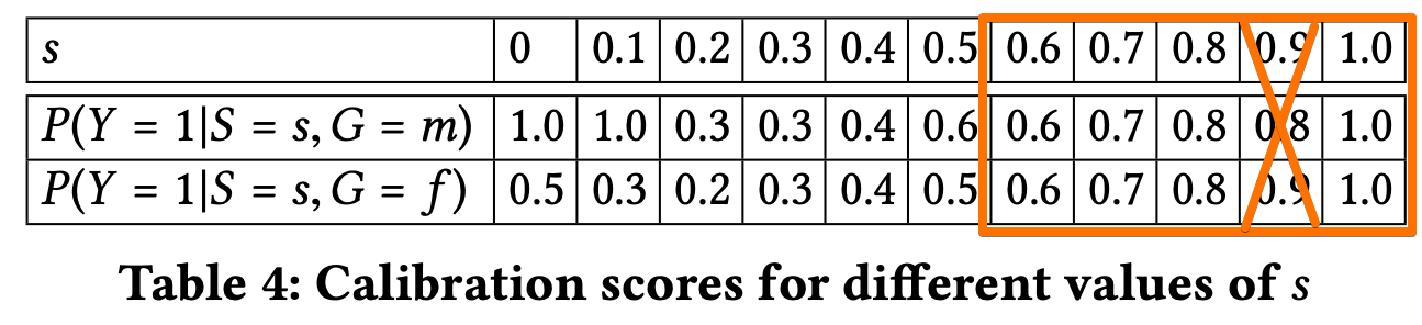
A classifier satisfies this definition if for any predicted probability score $S$, subjects in both protected and unprotected groups have equal probability to truly belong to the positive class.
\(P(Y = 1|S = s,G = m) = P(Y = 1|S = s,G = f )\) where,
© Verma et al.,
- Table 4 shows the scores for male and female applicants in each bin. The scores are quite different for lower values of S and become closer for values greater than 0.5. Thus, classifier satisfies the definition for high predicted probability scores but does not satisfy it for low scores.
- This is consistent with previous results showing that it is more likely for a male applicant with a bad predicted credit score (low values of S) to actually have a good score (definition 3.2.5), but applicants with a good predicted credit score (high values of S) have an equivalent chance to indeed have a good credit score, regardless of their gender (definition 3.2.1).
\(P(Y = 1|S = s,G = m) = P(Y = 1|S = s,G = f ) = s\) where,
© Verma et al.,
- According to Table 4., classifier is well-calibrated only for $s ≥ 0.6$. Classifier is deem to be partially satisfing this fairness definition.
\(E(S |Y = 1, G = m) = E(S |Y = 1, G = f ).\) where,
- Classifier is deemed to be satisfying this notion of fairness.
- This result further supports and is consistent with the result for equal opportunity (3.2.3), which states that the classifier will apply equivalent treatment to male and female applicants with actual good credit score ($TPR$ of 0.86).
On average, male candidates who actually have bad credit score receive higher predicted probability scores than female candidates. Classifier fails in satisfying this definition of fairness.
A classifier satisfies this definition if it produces the same classification for any two subjects with the exact same attributes $X$. which is,
\[(X_f =X_m ∧ G_f !=G_m)→d_f =d_m\]where,
Classifier fails in satisfying this definition
A classifier satisfies this definition if no sensitive attributes $S$ are explicitly used in the decision-making process,
where,
Classifier satisfies this definition
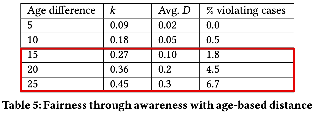
fairness is achieved if, \(D(M(x),M(y)) ≤ k(x,y)\)
where,
For example, mapping and distance metric can be defined as below.
$k = \begin{cases}
0 &\text{if attributes in X (all attributes other than gender) are identical }
1 &\text{otw}
\end{cases}$
and
$D = \begin{cases}
0 &\text{if classifier resulted in the same prediction}
1 &\text{otw}
\end{cases}$
or
$D(i, j) = S(i) - S(j)$
© Verma et al.,
For a smaller age difference, the classifier satisfied this fairness definition, but that was not the case for an age difference of more than 10 years.
© Verma et al.,
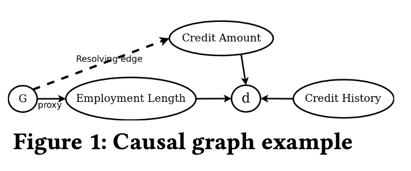
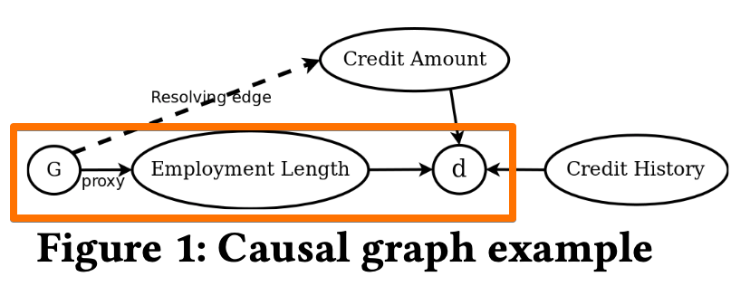
A causal graph is counterfactually fair if the predicted outcome $d$ in the graph does not depend on a descendant of the protected attribute $G$.
© Verma et al.,
$d$ is a dependent on credit history, credit amount, and employment length. Employment length is a direct descendant of $G$, hence, the given causal model is not counterfactually fair.
A causal graph has no unresolved discrimination if
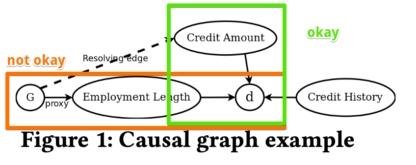
© Verma et al.,
- The path from $G$ to $d$ via credit amount is non-discriminatory as the credit amount is a resolving attribute
- But, the path via employment length(path from $G$) is discriminatory.
- Hence, this graph exhibits unresolved discrimination.
A causal graph is free of proxy discrimination if there exists no path from the protected attribute $G$ to the predicted outcome $d$ that is blocked by a proxy variable.
© Verma et al.,
- There is an indirect path from $G$ to $d$ via proxy attribute employment length.
- Thus, this graph exhibits proxy discrimination.
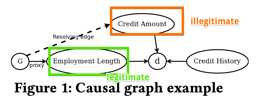
This definition classifies paths in a causal graph as legitimate or illegitimate.
© Verma et al.,
The End.
Non-designer designs the design of laboratory’s symbol, interestingly.
How to Use GSDS GPU Server
Fairness Definitions Explained
Fairness ML is the remedy for human’s cognition toward AI
과학자의 자세
미션: Shell 운용하는와중에 구글 검색하느라 시간 버리지 않기
Life Advice by Tim Minchin / 이번생을 조금이나마 의미있게 살고자
TensorflowLite & Coral Arsenal
Hivemapper,a decentralized mapping network that enables monitoring and autonomous navigation without the need for expensive sensors, aircraft, or satellites.
AMP Robotics, AI Robotics Company
자율주행 자동차 스타트업 오로라
Here I explore Aurora, tech company founded by Chris Urmson
Unpaired Image-to-Image Translation using Cycle-Consistent Adversarial Networks
미국의 AI 스타트업 50곳
2014 mid 맥북프로에 리눅스 얹기
Sparse Encoder, one of the best functioning AutoEncoder
Basic Concept of NN by formulas
싱글뷰 이미지로 다차원뷰를 가지는 3D 객체를 생성하는 모델
고통의 코랄 셋업(맥북)
HTML 무기고(GFM방식)