[CV][GAN][EN]Cycle GAN

I sometimes call cycleGAN “model” in this post.

0. Found at

Paper
Torch

1. Introduction

(upper left) Claude Monet(French, 1840-1926) placed his easel by the bank of Seine in lovely spring day. As the conveyer of “impression” , he depicted the color reflected by ligh shown to human eyes. He expressed impression of the theme through wispy brush strokes and a bright palette.
What if, Claude draws the same scene in summer night? We want to render the scene perhaps in pastel shades, with abrupt dabs of paint and a somewhat flattened dynamic range.

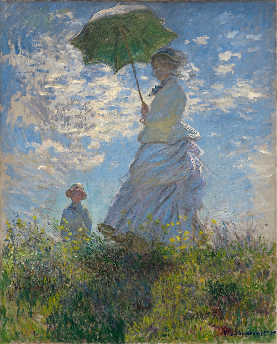
“La Promenade, Woman with a Parasol - Madame Monet and Her Son” by Claude Monet”

For this, we present a method that can learn to do the same: capturing special characteristics of one image collection and figuring out how these characteristics could be translated into the other image collection, in the absence of paired training examples; This is called image-to-image translation. Years of research in computer vision, image processing, computational photography and graphics have power translation system in the Supervised Settings where example image pairs ${x_i, y_i}_{i=1}^N$ are available.
However, obtaining paired training data can be difficult and expensive

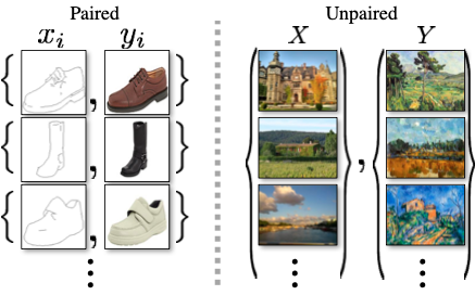
(Left): When ${ x_i, y_i}_{i=1}^N$ exist (Right): When just $x$ set and $y$ set exist
We therefore seek an algorithm that can learn to translate between domains without paired input-output examples. Assuming there is some underlying relationship between domains without paired input-output examples.
That is, instead of pairing $x_1$ to $y_1$, $x_2$ to $y_2$, we set ‘domain $X$’ and ‘domain $Y$’ by given set of images.

Render from $X$ to $Y$: Function $G$ is used
Render from $Y$ to $X$: Function $F$ is used. Thus, we set bi-directional two functions
Idea is that $G(X) = \hat{y} , x \in X $ is indistinguishable from images $y \in Y$ by an adversary trained to classify $\hat{y}$ apart from $y$.
Adversarial Loss: $G$ produces the output distribution over $\hat{y}$ that matches empirical distribution $p_{data}(y) $ (This requires $G$ to be stocastic).
Optimal $G$ translates the domain $X$ to domain $\hat{Y}$
But, still, there are many mapping $G$ that will induce the same distribution over $\hat{y}$. It is vulnerable to “mode collapse”, where all input images map to the same output image and the optimization fails to make progress
To relieve this, the property called ‘Cycle Consistency Loss’ was added.
If we translate sentence from Korean to English and then translate back it from English to Korean, we should arrive back at the original sentence.

(Left) forward cycle-consistency loss, math : $x\to G(x) \to F(G(x)) \approx x$
(Right) backward cycle-consistency loss, math : $y \to F(y) \to G(F(y)) \approx y$
We apply this structural assumption by training both the mapping G and F simultaneously, and adding a cycle consistency loss that encourages $F (G(x)) \approx x$ and $G(F(y)) \approx y$

GAN (Generative Adversarial Networks)
Image-to-Image Translation - pix2pix
Unpaired Image-to-Image Translation -CoGAN
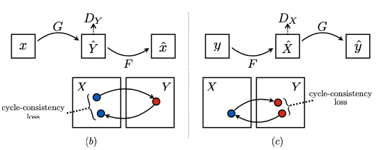
Cycle Consistency
Neural Style Transfer - synthesizing image using Gram matrix statistics of pre-trained deep features.

3. Formulation

3.0. Notation and Definition

3.0.1. Goal / Notation

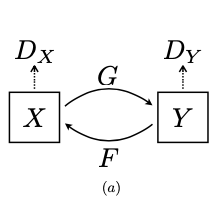
Goal : to learn mapping between two domains $X$ and $Y$.
Training Samples : ${ x_i, y_i}_{i=1}^N$ where $x_i\in X$ and $y_i\in Y$
Data Distribution : $x \sim p_{data}(x)$ $y \sim p_{data}(y)$
Mappings : $G:X \to Y$ and $F:Y \to X$
Adversarial Discriminators : $D_X$ and $D_Y$

3.0.2. Loss

Adversarial Loss : matching the distribution of generated images to the data distribution in the target domain
Cycle Consistencty Loss : prevent the learned mappings G and F from contradicting each other

3.1. Adversarial Loss

\[\tag{1} \mathcal{L}_{GAN}(G, D_Y, X, Y) = \mathbb{E}_{y \sim p_{data}(y)}[\log D_Y (y)] + \mathbb{E}_{x \sim p_{data}(x)}[1- \log D_Y (G(x))]\]

$G$ :
- Tries to generate image $G(x)$ that looks similar to images from donmain $Y$
- Aims to minimize this objective against an adversary $D$ that tries to maximize it
$D_Y$ : Aims to distinguish between translated samples $G(x)$ and real samples $y$

$\to$ i.e., “$min_G max_{D_Y} \mathcal{L}_{GAN} (G, D_Y, X, Y)$”

the same applies to mapping $F$:

$\to$ i.e., “$min_F max_{D_X} \mathcal{L}_{GAN} (F, D_X, Y, X)$”

3.2. Cycle Consistency Loss

With large enough capacity, a network can map the same set of input images to any random permutation of images in the target domain, where any of the learned mappings can induce an output distribution that matches the target distribution.
Thus, adversarial losses alone cannot guarantee that the learned function can map an individual input $x_i$ to a desired output $y_i$.
So “Cycle Consistency Loss” added to enhance individuality(mapping an individual input $x_i$ to a desired output $y_i$ well).

Here we will add forward cycle loss and backward cycle loss.
Math can show

\[\mathcal{L}(G,F) = \mathbb{E} _ {x \sim p_{data(x)}} \lbrack \lvert F(G(x)) - x\rvert _1 \rbrack + \mathbb{E} _ {y \sim p_{data(y)}} \lbrack \lvert G(F(y)) - y\rvert _1 \rbrack\]

3.3. Full Objective

Full Objective is

\[\mathcal{L}(G, F, D_X, D_Y) = \mathcal{L}_{GAN}(G, D_Y, X, Y) + \mathcal{L}_{GAN}(F, D_X, Y, X) + \lambda \mathcal{L}_{cyc}(G,F)\]

where $\lambda$ controls the relative importance of the two objs. Here, we aim to solve $G^*, F^* = \arg min_{G,F} max_{D_X, D_Y} \mathcal{L}(G,F,D_X,D_Y)$

To easily understand we learn one autoencoder $F \circ G: X \to X$ jointly with another $G \circ F: Y \to Y$

4. Implementation

4.1. Network Architecture

2 Stride Convolutions
2 Fractionally strided Convolutions (stride $\frac{1}{2}$)
6 Blocks for 128 X 128 images
9 Blocks for 256 X 256 images and higher resolition
Instance Normalization applied

Discriminator Networks

70 X 70 PatchGANs
- Aims classifiy whether 70 X 70 overlapping image patches are real or fake.

4.2. Training Details

For a GAN loss $\mathcal{L}_{GAN}(G,D,X,Y)$,
- Train the $G$ to minimize $\mathbb{E}_{x \sim p_{data}(x)}[(D(G(x)) -1)^2]$
- Train the $D$ to minimize $\mathbb{E}_{y \sim p_{data}(y)}[(D(Y) -1)^2] + \mathbb{E}_{x \sim p_{data}(x)}[D(G(x))^2]$
Reduct model oscillation, we updated the discriminators using a history of generated images rather than the ones produced by the latest generators. We keep an image buffer that stores the 50 previously created images.

5. Results

5.1. Evaluation

5.1.1. Evaluation Metrics

AMT perceptual studies
- Run real vs fake perceptual studies in Amazon Mechanical Turk(AMT)
- Participants were shown a sequence of pairs of images, one a real photo or map and one fake (generated by our algorithm or a baseline), and asked to click on the image they thought was real.
- The first 10 trials of each session were practice and feedback was given as to whether the participant’s response was correct or incorrect. The remaining 40 trials were used to assess the rate at which each algorithm fooled participants.
FCN Score
- Rather than perceptual studies, considered the gold standard for assessing graphical realism, we also seek an automative quanitative measure that does not require human experiment.
- FCN evalutes how interpretable the generated photos are according to an off-the-shelf semantic segmentation algorithm
- The intuition is that if we generate a photo from a label map of “car on the road”, then we have succeeded if the FCN applied to the generated photo detects “car on the road”
Semantic segmentation metrics
- Standard metrics from the Cityscapes benchmark(per-pixel accuracy, per-class accuracy, and mean class Intersection-Over-Union (Class IOU))

5.1.2. Baselines

CoGAN
SimGAN
Feature loss + GAN
BiGAN/ALI
pix2pix

5.1.3. Comparison against Baselines

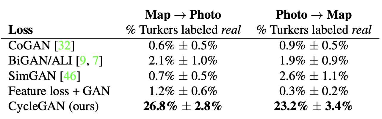
Table shows performance regarding AMT perceptual realism task(human participatant gauge the performance)
cycleGAN can fool participants on around a quarter of trials while other baselines almost never fooled participants

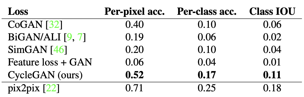
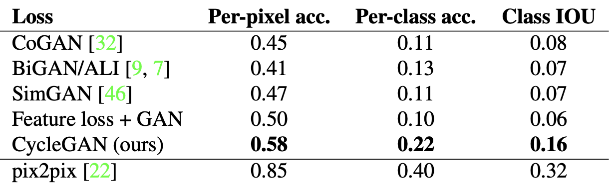
Table shows the performance of the labels → photo task on the Cityscapes
cycleGAN outperforms the baselines.

Table evaluates the opposite mapping (photos→labels).
cycleGAN outperforms the baselines.

5.1.4. Loss Function Analysis

5.1.4.1. Abalation Studies(Quantative)

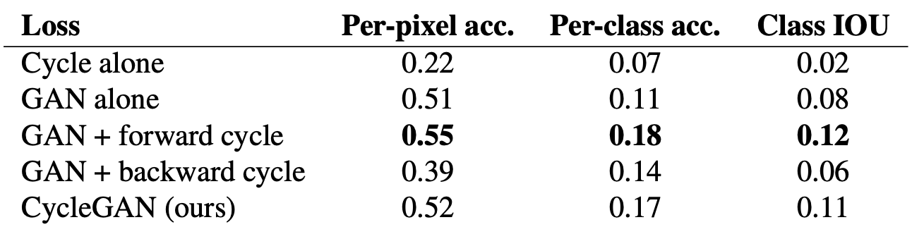
evaluated on Cityscapes labels → photo

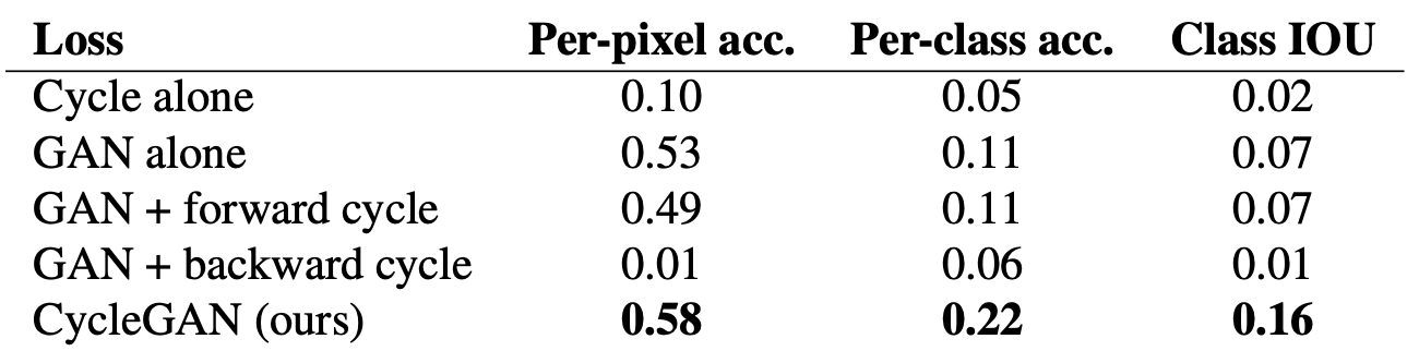
evaluated on Cityscapes photo → labels

Analysis

Removing GAN loss degrades the rsults.
Cycle loss in one-direction shows instability of performance: Like,
- GAN + forward cycle loss denoted as $\mathbb{E} _ {x \sim p_{data(x)}} \lbrack \lvert F(G(x)) - x\rvert _1 \rbrack$
- GAN + backward cycle loss denoted as $\mathbb{E} _ {y \sim p_{data(y)}} \lbrack \lvert G(F(y)) - y\rvert _1 \rbrack$

5.1.4.2. Qualitative

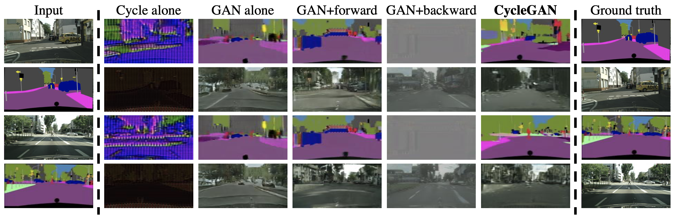
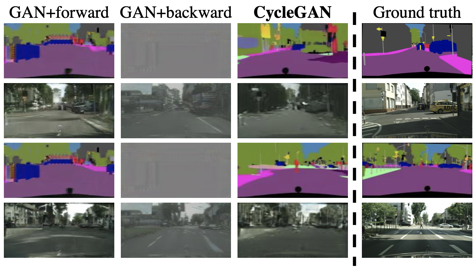
Cycle loss in one-direction shows instability of performance: Performs poorly only in one cycle. Importantce of Cycle Consistency Loss can be known here.
Especially GAN+Forward,

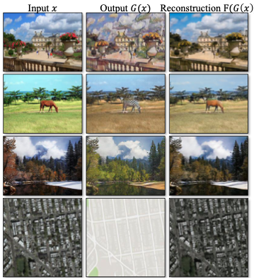
5.1.5. Image reconstruction quality

Few sample of reconstructed images, which is $F(G(X))$, show almost similar images, even close to original images $X$.

5.2. Applications

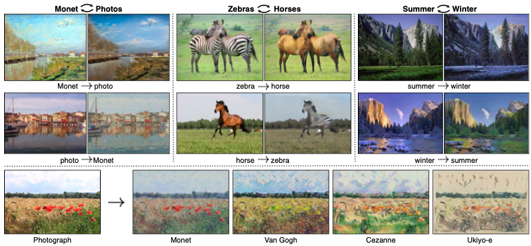
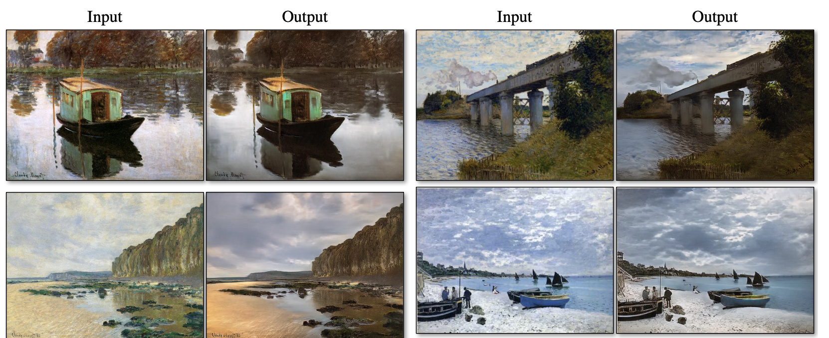
Collection style transfer
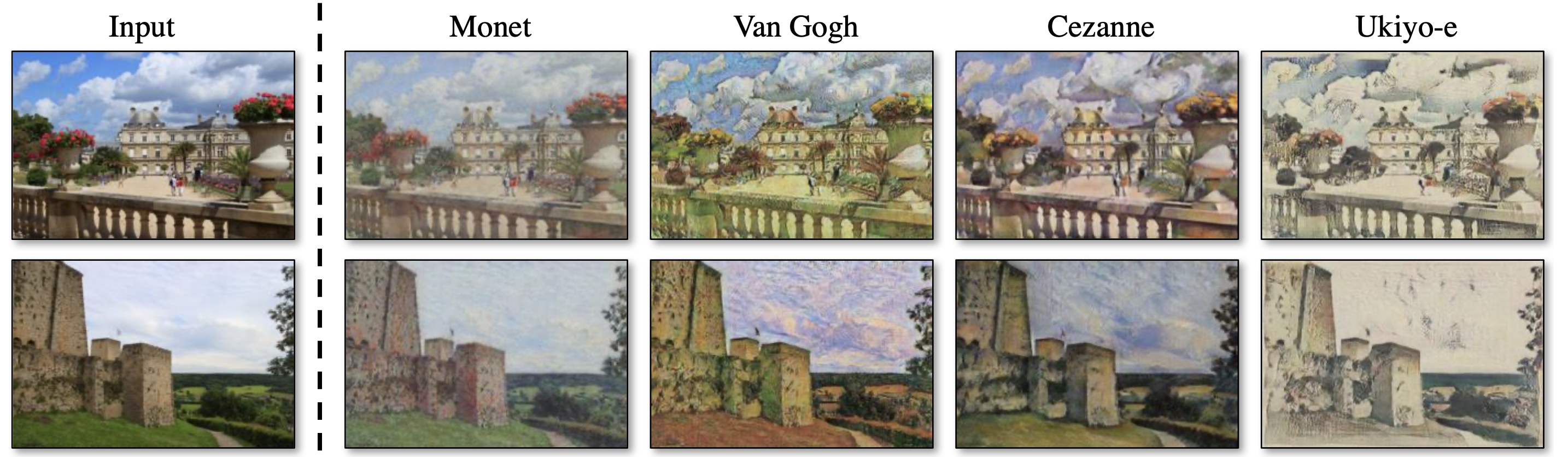
- Learns to mimic the style of an entire collection of artworks, rather than transferring the style of a single selected piece of art.
- Therefore, we can learn to generate photos in the style of, e.g., Van Gogh, rather than just in the style of Starry Night.
- The size of the dataset for each artist/style was 526, 1073, 400, and 563 for Cezanne, Monet, Van Gogh, and Ukiyo-e.
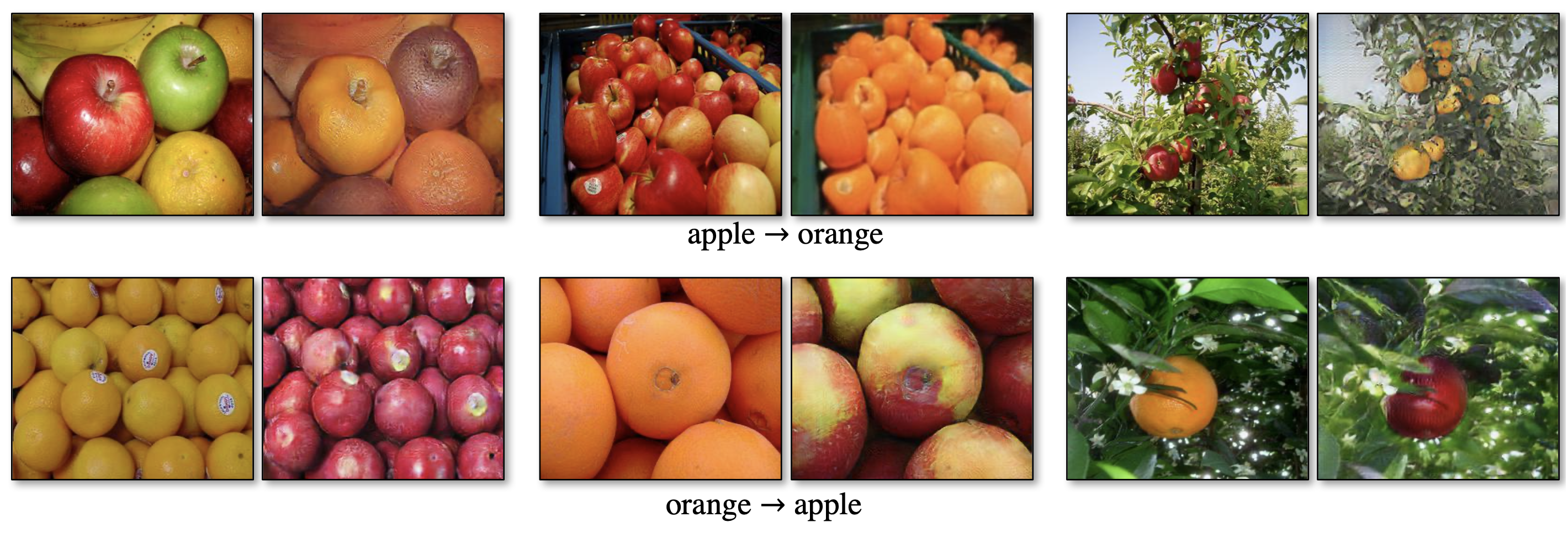
Object transfiguration
- Data from ImageNet
Season transfer
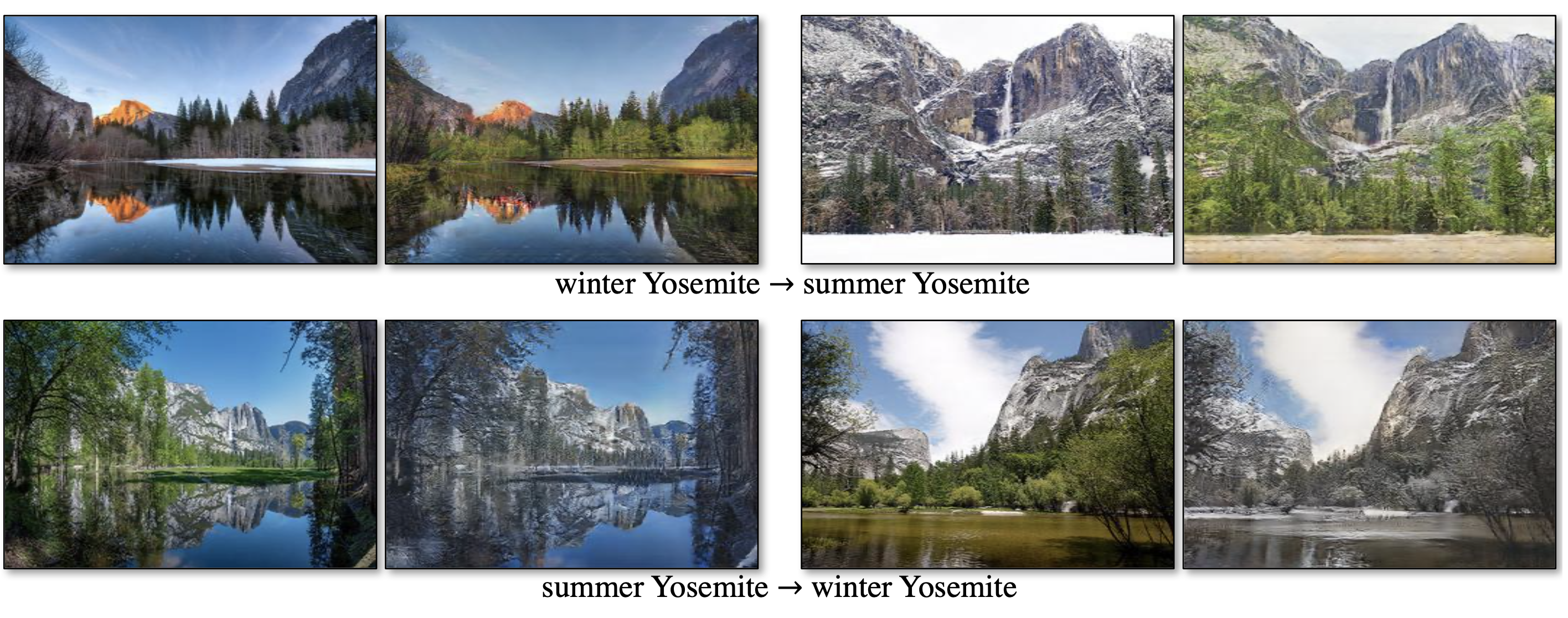
- Model learned on 854 winter photos and 1273 summer photos of Yosemite downloaded from Flickr.
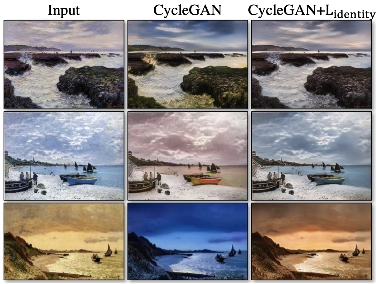
Photo generation from paintings
- from paining to photo, one more loss function practically added. It is called “Identity Mapping Loss” denoted as, $\mathcal{L}_{identity}(G,F) = \mathbb{E} _ {y \sim p_{data(y)}} \lbrack \lvert G(y) - y\rvert _1 \rbrack + \mathbb{E} _ {x \sim p_{data(x)}} \lbrack \lvert F(x) - x\rvert _1 \rbrack$
- This loss encourages the mapping to preserve color composition between the input and output.
- The effect of Identity Mapping Loss can be seen below.
Photo enhancement
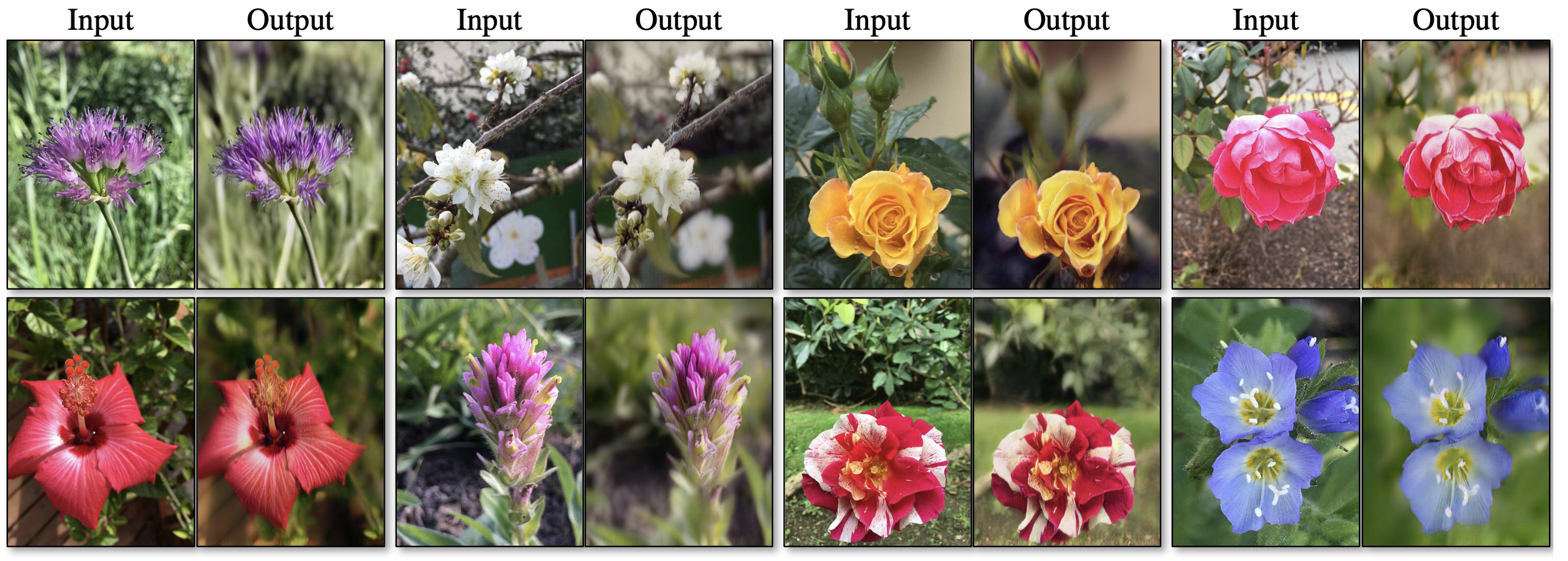
- Model successfully generates photos with shallower depth of field from the photos taken by smartphones.
- Method can be used to generate photos with shallower depth of field.
- Smartphones have small aperature(Deep DoF) while DSLRs have large aperture(Shallow DoF).
- Shallower DoF was expressed through the model.

6. Limitations and Discussion

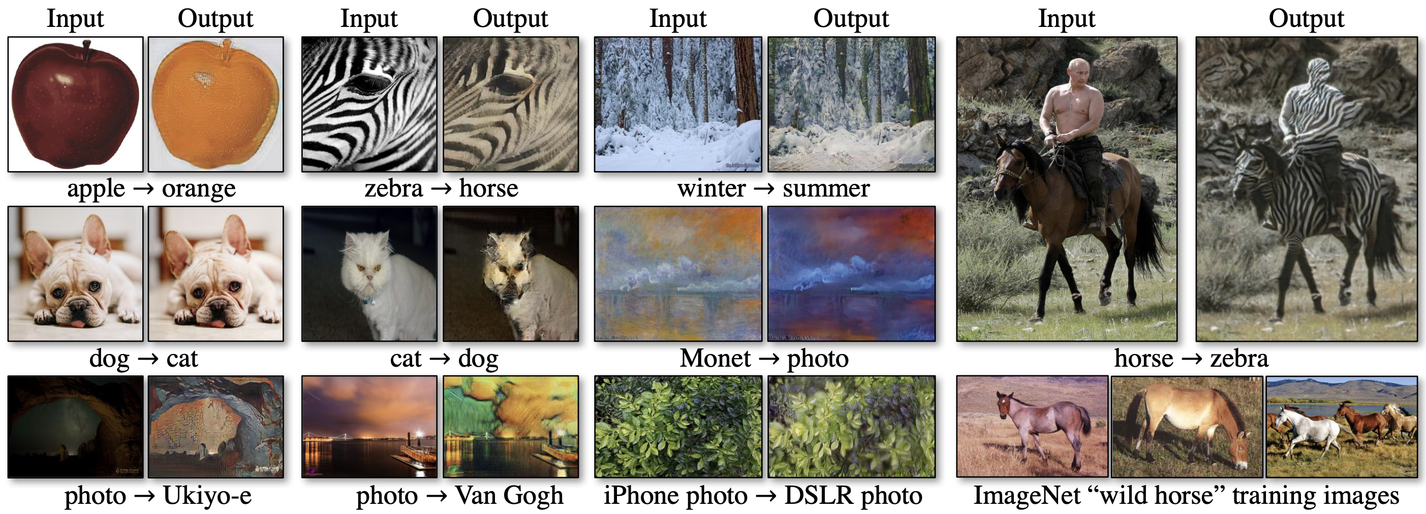
dog → cat : performs poorly
zebra → horse : performs poorly
winter → summer : still, output is like winter
horse → zebra : zebra is riding zebra etc..

BUT

Nonetheless, in many cases completely unpaired data is plentifully available and should be made use of. This paper pushes the boundaries of what is possible in this “unsupervised” setting.

The End.

2020 21